SLAP2 Utils Example Notebook

This notebook will highlight core features included in SLAP2_Utils. The example will demonstrate how to extract useful metadata, extract a trace signal, and use basic plotting. This will give users a better understanding of how to work with the library with their own data. For further information on any functions used in the notebook, please reference the documentation

Loading a Data File

Loading data from a SLAP2 binary file requires importing the DataFile class from the library. The coorsponding meta data file should be in the same directory with the same file name. If either of these conditions are not met, then an error will be thrown during loading

from slap2_utils.datafile import DataFile

binaryFilePath = "3DExampleScan.dat"
dataFile = DataFile(binaryFilePath)

Basic information about the acquisition is stored inside the file header. We can inspect this by accessing the header attribute in the datafile object. This attribute stores information inside a dictionary.

display(dataFile.header)

{'firstCycleOffsetBytes': 136.0,
 'lineHeaderSizeBytes': 40.0,
 'laserPathIdx': 0.0,
 'bytesPerCycle': 31270.0,
 'linesPerCycle': 302.0,
 'superPixelsPerCycle': 9595.0,
 'dmdPixelsPerRow': 1280.0,
 'dmdPixelsPerColumn': 800.0,
 'numChannels': 1.0,
 'channelMask': 1.0,
 'numSlices': 28.0,
 'channelsInterleave': 0.0,
 'fpgaSystemClock_Hz': 200000000.0,
 'referenceTimestamp_lower': 3670612649.0,
 'referenceTimestamp_upper': 197.0,
 'channels': [0],
 'referenceTimestamp': 849779169961,
 'file_version': 2,
 'magic_start': 322379495,
 'magic_end': 322379495}

If we wanted to access specific information stored in the header we can do so by using the corresponding key. For this simulated recording we can tell that simulated scan is a single channel volumetric recording with 28 slices.

print('Number of imaging planes: ', dataFile.header['numSlices'], '\nList of recorded channels :',dataFile.header['channels'])

Number of imaging planes:  28.0
List of recorded channels : [0]

Inspecting Acquisition Metadata

Once loaded into Python, the acquisition metadata is stored in the MetaData subclass of the DataFile object. This object has more detailed information about the microscope settings during the acquisition.

# Here is an example of import data stored in the `MetaData` object
print('The laser AOM was set to: ', dataFile.metaData.aomVoltage)
print('The duration of the acquisition was', dataFile.metaData.acqDuration_s, 'secs')

The laser AOM was set to:  1.9500000000000002
The duration of the acquisition was 10.0 secs

The MetaData object is the parent object of other objects, such as the AcquisitionContainer, which stores a list of all regions of interest (ROI). Information for each ROI is stored in slapROI objects. Now we’ll look at how to pull out this information

print('The number of ROIs in the acquistion is: ', len(dataFile.metaData.AcquisitionContainer.ROIs))

The number of ROIs in the acquistion is:  643

Let’s look at the information stored in a slapROI object.

• slapROI.imageMode: SLAP2 has two types of ROIs, raster and integrated

• slapROI.roiType: ROI shapes can be rectangular or arbitrary

• slapROI.shapeData: Arbitrary ROI shapes are stored in a series of coordinates

• slapROI.z: The remote focusing positiion is stored in the z attribute

‘slapROI’ documentation

print("ROI Imaging Mode: ", dataFile.metaData.AcquisitionContainer.ROIs[0].imageMode, "\n")
print("ROI Type: ", dataFile.metaData.AcquisitionContainer.ROIs[0].roiType, "\n")
print("Shape Data: ", dataFile.metaData.AcquisitionContainer.ROIs[0].shapeData, "\n")
print("Remote focusing position (um): ", dataFile.metaData.AcquisitionContainer.ROIs[0].z, "\n")

ROI Imaging Mode:  Integrate

ROI Type:  ArbitraryRoi

Shape Data:  [[375. 376. 374. 375. 376. 377. 374. 375. 376. 377. 374. 375. 376. 375.]
 [716. 716. 717. 717. 717. 717. 718. 718. 718. 718. 719. 719. 719. 720.]]

Remote focusing position (um):  229.0

‘SLAP2_Utils’ has inbuilt utils for interacting with ROI shape data which may be useful for users building analysis or visualization pipelines. These are stored in slap2_utils.utils.roi_utils. Let’s look at these functions

from slap2_utils.utils import roi_utils
import matplotlib.pyplot as plt
import numpy as np

roi_utils.roiImg will return a 2D array of the optical plane the ROI is in (slapROI.z). Pixels belonging to the ROI will be set to the value one, while the other pixels will be set to a value of 0.

`roi_utils.roiBoolean’ returns the same data but as a boolean, which is useful for generating activity traces

`roi_utils.roiLabels’ returns either a 2D or 3D label array, representing each ROI as an integer. An option argument is a path of a SLAP2 reference TIF file, which will match the ROI position in Z to image slices in the volumetric TIF file.

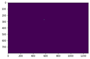
# Plotting the pixels belonging to the ROI at index 10 in dataFile.metaData.AcquisitionContainer.ROIs
roi_utils.roiImg(dataFile, 10)
plt.imshow(roi_utils.roiImg(dataFile, 10))
plt.show()

# The same data in an boolean array
print(np.unique(roi_utils.roiBoolean(dataFile, 10)))

[False  True]

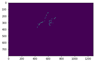
# Ploting all the ROIs on a particular plane of the acquisition
roiLabelArray = roi_utils.roiLabels(dataFile)
plt.imshow(roiLabelArray[15, :, :])
plt.show()

Plotting

SLAP2_Utils has a few basic plotting features to better visualize the data in ROIs

from slap2_utils.utils.plots import slap2Plots

# We can plot the contours of a given ROI over a reference image
# This simulated data does not have a reference image, so we will use an array of zero
slap2Plots.roiOverlay(dataFile, np.zeros_like(roiLabelArray), 15)

<Axes: >

Trace Extraction

Trace extraction can be handled directly using the Trace object. However, SLAP2_Utils includes helper functions to streamline this process further.

from slap2_utils.utils import trace
from slap2_utils.functions import tracefunctions

# Let's extract a trace for ROI 15
# we need to get determine what channel, there is only one in this simulated recording
chIdx = 1
# We need to find the ROI's Z position in the fastz of the DataFile
roi15 = dataFile.metaData.AcquisitionContainer.ROIs[15]
zIdx = dataFile.fastZs.index(roi15.z)



# Can now initialize the Trace object
Trace = trace.Trace(dataFile, zIdx, chIdx)

# We need to set the pixel mask for Trace generation
roi15Mask = roi_utils.roiBoolean(dataFile, 15)

# Exclude any raster-mode pixels
rasterPixels = None

Trace.setPixelIdxs(rasterPixels, roi15Mask)

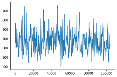
#We can smooth the trace with temporal weights
print('The trace smoothed with a weighted average')
trace15, sumDataWeighted, sumExpected, sumExpectedWeighted  = Trace.process(150, 1000)
plt.plot(trace15)
plt.show()

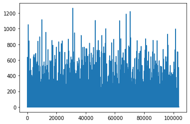
# Or we can set the weighted windows to 1 and return the raw trace
print('The raw trace')
rawtrace15, sumDataWeighted, sumExpected, sumExpectedWeighted  = Trace.process(1, 1)
plt.plot(rawtrace15)
plt.show()

# Traces from volumetric acquisitions need to be further processed to remove times when the microscope was focused on a different plane
print('The raw trace cleaned to include only data corresponding the correct axial focus')
volumetricTrace15 = tracefunctions.cleanVolumeTrace(dataFile, zIdx, rawtrace15)
plt.plot(volumetricTrace15)
plt.show()

The trace smoothed with a weighted average

The raw trace

The raw trace cleaned to include only data corresponding the correct axial focus

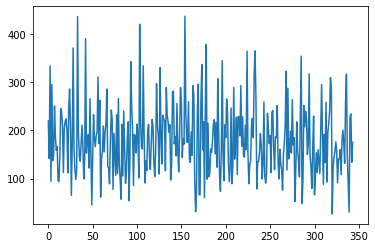
All of these steps can excuted using the returnVolumeTrace function

# Returning the raw trace for the ROI with one line
rawTrace15, volumeTrace15 = tracefunctions.returnVolumeTrace(dataFile, 15)
plt.plot(volumeTrace15)
plt.show()

Extracting Line Data

The ‘getLineData’ can be used to return the recorded data for a specific index, cycle, and channel

dataFile.getLineData(1, 2)

[array([], shape=(0, 1), dtype=int16)]